In a previous vignette (Building Up a Dataset for the Study of Phosphoserines) we showed how to proceed in order to build a dataset containing information regarding the serine residues from the human phosphoproteome. Herein, we will download such a dataset, which will be use as a starting point to test the following working hypothesis:
Regulatory phosphoserines have a differential sequence environment with respect to non-regulatory phosphoserines.
Therefore, the null hypothesis can be stated as that the neighboring amino acids around non-regulatory and regulatory phosphoserines do not differ. The alternative hypothesis is that there are specific amino acids at specific positions (around the phosphosite) that are avoided in the neighborhood of regulatory sites (significantly lower frequencies in the environments of regulatory phosphoserines with respect to their non-regulatory counterpart), while other amino acids at specific positions could be preferred in the neighborhood of regulatory phosphoserines (significantly higher frequencies in the environments of regulatory phosphoserines with respect to their non-regulatory counterpart).
The reader interested in the details about how the data that will allow us to test this hypothesis were collected, can visit the above referred vignette.
url <- "https://github.com/jcaledo/ptm_db/raw/master/SerSites.Rda"

destfile <- tempfile(pattern = 'all',
                     tmpdir = tempdir(),
                     fileext = '.Rda')
download.file(url, destfile, quiet = TRUE)
load(destfile)
The above chunk will load in your global environment of R a dataframe named ‘serine_sites’ that looks like:
serine_sites[1:10, ]
##        id pos pSer regulatory                   env
## 2  P31946  39 TRUE      FALSE KAVTEQGHELsNEERNLLSVA
## 3  P31946  47 TRUE      FALSE ELSNEERNLLsVAYKNVVGAR
## 4  P31946  59 TRUE      FALSE AYKNVVGARRsSWRVISSIEQ
## 5  P31946  60 TRUE      FALSE YKNVVGARRSsWRVISSIEQK
## 6  P31946  66 TRUE      FALSE ARRSSWRVISsIEQKTERNEK
## 7  P31946 116 TRUE      FALSE YLIPNATQPEsKVFYLKMKGD
## 8  P31946 132 TRUE      FALSE KMKGDYFRYLsEVASGDNKQT
## 9  P31946 136 TRUE      FALSE DYFRYLSEVAsGDNKQTTVSN
## 10 P31946 186 TRUE       TRUE FSVFYYEILNsPEKACSLAKT
## 11 P31946 212 TRUE      FALSE IAELDTLNEEsYKDSTLIMQL
Each row corresponds to a serine site from the human phosphoproteome and the columns are:
- id: UniProt ID of the phosphoprotein.
- pos: Position of the serine residue in the primary structure of the protein.
- pSer: Whether or not the serine is phosphorylatable.
- regulatory: Whether or not the serine has been described as regulatory.
- env: Sequence environment (flanking amino acids at positions from –10 to +10 relative to the central Ser).
As you can observe, we have collected tens of thousands of phospho-serine sites in this dataset. However, as pointed out by Gustav E. Lienhard, there are reasons for believing that some portion of these reported phosphorylations might have little or no functional importance. Thus, we are going to use an astringent criterion to label a phosphosite as regulatory: it should have been empirically proved that the phosphorylation of that site has a regulatory effect on the phosphoprotein. To search for those phosphosites fulfilling such criterion, we made use of the function reg.scan().
At this point we are interested in addressing whether or not the sequence environments of those phospho-serines that have been described as playing a regulatory function, can be statistically distinguished from those environments belonging to phospho-serines detected in high-throughput analyses, but for which we have no information about their biological relevance.
Amino acid frequencies within environments
Our first task toward our goal is to compute the amino acid frequencies at each position within the environment of regulatory and non-regulatory pSer. For each serine site, the frequency of flanking amino acids at each position from –10 to +10 relative to the central Ser is recorded making use of env.matrices(). The only argument that this function takes is a vector containing the environments as character string.
Non regulatory pSer sites
non_reg_pSer <- env.matrices(serine_sites$env[which(serine_sites$pSer == TRUE & serine_sites$regulatory == FALSE)])
The environments matrix:
environments_non_reg_pSer <- non_reg_pSer[[1]]
head(environments_non_reg_pSer)
##                       -10 -9 -8 -7 -6 -5 -4 -3 -2 -1 0 1 2 3 4 5 6 7 8 9 10
## KAVTEQGHELsNEERNLLSVA   K  A  V  T  E  Q  G  H  E  L s N E E R N L L S V  A
## ELSNEERNLLsVAYKNVVGAR   E  L  S  N  E  E  R  N  L  L s V A Y K N V V G A  R
## AYKNVVGARRsSWRVISSIEQ   A  Y  K  N  V  V  G  A  R  R s S W R V I S S I E  Q
## YKNVVGARRSsWRVISSIEQK   Y  K  N  V  V  G  A  R  R  S s W R V I S S I E Q  K
## ARRSSWRVISsIEQKTERNEK   A  R  R  S  S  W  R  V  I  S s I E Q K T E R N E  K
## YLIPNATQPEsKVFYLKMKGD   Y  L  I  P  N  A  T  Q  P  E s K V F Y L K M K G  D
and its frequencies matrix:
freq_non_reg_pSer <- non_reg_pSer[[2]]
head(freq_non_reg_pSer)
##    -10   -9   -8   -7   -6   -5   -4   -3   -2    -1 0    1     2     3     4     5    6    7
## A 9011 8805 8887 8992 8924 8869 8679 8222 8799  9112 0 6974  8262  8248  8529  8517 8854 8875
## C 1766 1866 1979 1679 1721 1610 1469 1452 1651  1758 0 1483  1551  1434  1589  1529 1606 1737
## D 6267 6125 6036 6300 6145 6066 6373 6223 6282  7873 0 7149  7899  7812  6892  6980 6541 6787
## E 9724 9761 9547 9661 9372 8845 9188 8339 8201  7081 0 8225 11367 12373 10127 10059 9898 9904
## F 3217 3174 3239 3091 3190 3526 3310 3011 3088  3739 0 4092  2766  3015  3142  3193 3281 3271
## G 8843 8734 8688 9232 8897 8661 9319 8705 8576 11382 0 8531  9684  9451  8454  8447 8686 8628
##       8    9    10
## A  8748 8808  8911
## C  1631 1656  1886
## D  6674 6525  6577
## E 10095 9981 10213
## F  3317 3182  3239
## G  8632 8696  8680
Regulatory pSer sites
reg_pSer <- env.matrices(serine_sites$env[which(serine_sites$pSer == TRUE & serine_sites$regulatory == TRUE)])
The environments matrix:
environments_reg_pSer <- reg_pSer[[1]]
head(environments_reg_pSer)
##                       -10 -9 -8 -7 -6 -5 -4 -3 -2 -1 0 1 2 3 4 5 6 7 8 9 10
## FSVFYYEILNsPEKACSLAKT   F  S  V  F  Y  Y  E  I  L  N s P E K A C S L A K  T
## YKNVVGARRSsWRVISSIEQK   Y  K  N  V  V  G  A  R  R  S s W R V I S S I E Q  K
## WRVLSSIEQKsNEEGSEEKGP   W  R  V  L  S  S  I  E  Q  K s N E E G S E E K G  P
## SIEQKSNEEGsEEKGPEVREY   S  I  E  Q  K  S  N  E  E  G s E E K G P E V R E  Y
## FSVFHYEIANsPEEAISLAKT   F  S  V  F  H  Y  E  I  A  N s P E E A I S L A K  T
## YKNVVGARRSsWRVVSSIEQK   Y  K  N  V  V  G  A  R  R  S s W R V V S S I E Q  K
and its frequencies matrix:
freq_reg_pSer <- reg_pSer[[2]]
head(freq_reg_pSer)
##   -10  -9  -8  -7  -6  -5  -4  -3  -2  -1 0   1   2   3   4   5   6   7   8   9  10
## A 263 234 238 261 248 246 211 200 273 265 0 152 239 248 242 261 245 262 265 262 266
## C  50  38  61  48  38  51  42  31  54  39 0  25  54  52  41  50  47  48  48  72  45
## D 196 196 199 203 213 203 174 166 162 256 0 216 246 289 229 243 227 212 222 206 192
## E 281 294 260 253 282 226 298 187 196 181 0 214 303 392 266 316 318 313 309 288 299
## F 105 123 113 119 107  81 123 107  81 113 0 186  92  93 109 110  93 100 123 120  93
## G 278 275 269 286 256 230 258 243 184 308 0 167 260 276 269 238 240 258 253 256 269
Comparing regulatory and non-regulatory sequence environments: Z-tests
Since we are interested in detecting differences between the sequence environments of regulatory and non-regulatory pSer sites, we formulate the following null hypothesis: the difference between the relative frequency matrices (regulatory – non-regulatory) yields the zero matrix.
To contrast this hypothesis, a new matrix, 
freq_reg_pSer <- freq_reg_pSer[, -11]
freq_non_reg_pSer <- freq_non_reg_pSer[, -11]
Then, we can call the env.Ztest() as shown next:
Z <- env.Ztest(pos = freq_reg_pSer,
               ctr = freq_non_reg_pSer,
               alpha = 0.001)
This function returns a list with three elements. The first one (Z[[1]]) is the Z matrix. Each element from this matrix should follow a standardized normal distribution under the null hypothesis conditions.
head(Z[[1]])
##          -10         -9         -8         -7         -6         -5         -4         -3
## A -0.2223462 -1.7557211 -1.6383256 -0.3140007 -1.0320727 -1.0601668 -3.1821728 -3.0837692
## C -0.3134236 -2.7450962  0.3136926 -0.2378124 -2.0635736  0.4699045 -0.2217101 -2.1119963
## D  0.7691829  1.0733415  1.4708789  1.1856083  2.1758651  1.6790525 -1.1080273 -1.4110829
## E -0.4043270  0.3164107 -1.4159769 -2.0972770  0.2923735 -2.4029648  1.5621141 -4.3905795
## F  0.9616732  2.6393045  1.6219958  2.5393646  1.2241581 -2.5680789  2.2736349  1.7379265
## G  1.0101728  1.0290916  0.7500031  0.7842831 -0.4564346 -1.7525463 -1.1201505 -0.9454774
##           -2         -1          1          2          3          4          5           6
## A  0.7893408 -0.2835273 -4.4073160 -0.3539518  0.2614526 -0.6722881  0.5743696 -1.09832684
## C  0.6987925 -2.0523038 -3.6913228  1.0997351  1.3224666 -0.9265892  0.6708218 -0.07271864
## D -1.8806299  1.4771642  0.3139033  0.8037268  3.5038165  1.6919912  2.3929942  2.26644477
## E -3.3559219 -2.1306987 -2.0271204 -1.9578217  1.3693773 -2.0982761  1.0704360  1.45851852
## F -1.1422780  0.2265912  4.8376453  1.0612197  0.3956299  1.5419377  1.4864051 -0.41844018
## G -5.1627840 -1.6770630 -6.6109193 -1.6719712 -0.2183401  1.1821488 -0.7812983 -1.11092807
##            7           8           9         10
## A -0.0320318  0.39238706  0.09303330  0.1521416
## C -0.4830416 -0.03467653  2.71154666 -1.5885364
## D  0.7843950  1.67912058  0.91881989 -0.1851315
## E  1.1674071  0.60905939 -0.43610805 -0.1830799
## F  0.3246850  2.25482288  2.37340382 -0.2900308
## G  0.1778726 -0.14878272 -0.07737353  0.7647723
The second element, Z[[2]] is a dataframe containing those amino acid that make a significant contribution (according to the confidence level, alpha, chosen for the user) to the differential environment by being overrepresented in the environment of regulatory pSer.
head(Z[[2]])
##   aa at         Z       pValue
## 3  R -3 15.287005 0.000000e+00
## 7  P  1 11.886446 0.000000e+00
## 5  R -2 10.148514 0.000000e+00
## 2  R -5  5.002062 2.836021e-07
## 6  F  1  4.837645 6.569318e-07
## 8  R  2  3.506275 2.272129e-04
The third element is also a dataframe containing those other residues that make a significant contribution to the differential environment, but in this occasion being underrepresented in the environment of regulatory pSer.
head(Z[[3]])
##    aa at         Z       pValue
## 13  G  1 -6.610919 1.909703e-11
## 16  S  1 -6.430280 6.368451e-11
## 15  R  1 -5.777499 3.790956e-09
## 6   S -3 -5.645361 8.241752e-09
## 14  K  1 -5.356249 4.248366e-08
## 8   G -2 -5.162784 1.216519e-07
As you can see, we must reject the null hypothesis and declare that the sequence environments of regulatory and non-regulatory phospho-serine sites are statistically distinguishable.
Ploting the differences between sequence environment
The conclusion to which we have just arrived: the regulatory pSer sites exhibit a differential sequence environment, can be visually illustrated making use of the env.plot() function. For instance, let’s focus on proline and arginine, amino acids that are clearly overrepresented in the environment of regulatory pSer sites. On the other hand, glycine and serine are clearly underrepresented in the environment of regulatory pSer sites.
oldpar <- par()
par(mfrow=c(2,2))
on.exit(oldpar)

env.plot(Z = Z[[1]], aa = "P", pValue = 0.001, ylim = 'automatic')
env.plot(Z = Z[[1]], aa = "R", pValue = 0.001, ylim = 'automatic')
env.plot(Z = Z[[1]], aa = "G", pValue = 0.001, ylim = 'automatic')
env.plot(Z = Z[[1]], aa = "S", pValue = 0.001, ylim = 'automatic')
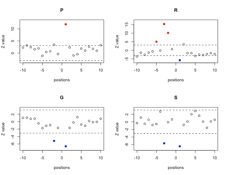
A Z-value (the ordinate variable) that is much greater than zero indicates that the analyzed amino acid is overrepresented at the indicated position (the abscissa variable). Conversely, a Z-value that is much less than zero indicates that the amino acid being analyzed is underrepresented at that position. The horizontal dashed lines delimit the 99.999 % confidence interval of the Z-statistic. Thus, we can confidently conclude that regulatory pSer environments exhibit a preference for proline at position +1 and for arginine at positions -2, -3 and -5. On the other hand, serine is avoided at position -3 and +1, while glycine is underrepresented at -2 and +1, arginine at the position +1 seems to be also excluded from the regulatory environments.
