Aim of this vignette
The goal of this document is to show how to coordinate multiple functions from the ptm package to address concrete questions, related with the sequence environment of sulfoxidation sites in proteins. Herein, we address whether those methionines prone to oxidation have a differential sequence environment with respect to their oxidation-resistant counterpart.
Background
Before addressing the problem we want to resolve, let me give you a little bit of background about methionine modification (the reader interested in getting a more thoroughly insight, is pointed to the reading Methionine in Proteins, which is an extract of the review Methionine in proteins: The Cinderella of the proteinogenic amino acids.
The oxidation of protein-bound methionine to form methionine sulfoxide (MetO), has traditionally been regarded as an oxidative damage. However, growing evidences support the view of this reversible reaction as a regulatory post-translational modification (PTM). The mere addition of an oxygen atom to the sulfur atom of methionine can cause changes in the physicochemical properties of the whole protein, which, in turn, can affect the stability and/or the activity of the oxidized protein. Thus, the oxidation of methionine residues to methionine sulfoxide both in vitro and in vivo has been reported to have multiple and varied implications for protein function.
The perception that methionine sulfoxidation may provide a mechanism to the redox regulation of a wide range of cellular processes, has stimulated numerous studies on this PTM in very diverse proteins. All this information has been gathered in a database: MetOSite. This database can be queried through a browser interface or, alternatively, it can be accessed programmatically by means of its API RESTful, as we will illustrate in the examples presented herein.
Comparison of sequence environments
Protein-bound methionines are not equally prone to oxidation. In fact, we have previously shown that methionine sulfoxidation does not follow a random pattern (Aledo et al. 2015). On the contrary, it can be verified that methionine oxidation is a sequence-dependent specific event. In few words, in the current tutorial we will show that those methionine sites prone to oxidation (MetO sites) and those others resistant to oxidation (Met sites) have different sequence environments.
The tools we are going to use
As stated earlier, the current document aims to illustrate how we can achieve our goal (show the existence of differential environments) in a straightforward and painless way! To this end, all we need to use are the following functions from the ptm package:
meto.search()env.extract()env.matrices()env.Ztest()env.plot()
Getting the data
The first is the first. If we are going to analyze data, we need first to obtain the data of interest. Let say that we are interested in MetO sites from human proteins oxidized in vivo by hydrogen peroxide and detected in high-throughput studies (HTS). So, how can we know what methionyl residues from the human proteome fulfill these conditions? Fortunately, obtaining such piece of information is going to be awfully easy using the function meto.search().
library(ptm)
data <- meto.search(highthroughput.group = TRUE,
                    bodyguard.group = FALSE,
                    regulatory.group = FALSE,
                    organism = 'Homo sapiens',
                    oxidant = 'H2O2')
| prot_id | prot_name | met_pos |
|---|---|---|
| A2RRP1 | Neuroblastoma-amplified sequence | 2042 |
| A2RRP1 | Neuroblastoma-amplified sequence | 2204 |
| A3KN83 | Protein strawberry notch homolog 1 | 1050 |
| A3KN83 | Protein strawberry notch homolog 1 | 167 |
| A5YKK6 | CCR4-NOT transcription complex subunit 1 | 1927 |
| A5YKK6 | CCR4-NOT transcription complex subunit 1 | 2361 |
| A5YKK6 | CCR4-NOT transcription complex subunit 1 | 2154 |
| A6NEC2 | Puromycin-sensitive aminopeptidase-like protein | 216 |
| A6NIZ1 | Ras-related protein Rap-1b-like protein | 111 |
| A8K0Z3 | WASH complex subunit 1 | 202 |
Observe that with the selected parameters that we have passed as arguments to the function, we obtain a dataframe with 4484 entries (MetO sites) and 7 variables. If we examine the data, we’ll be able to check that all the entries belong to human proteins, and the hydrogen peroxide is an oxidant for all these sites. Furthermore, we can make sure that all the sites have been detected in HTS (that is indicated by the variable reg-id = 1). That’s good because it means that everything has gone according to the expectation, but it is not surprising because we requested that by means of the arguments that we passed to the function meto.search(). However, the sagacious reader may have realized that at no time have we asked for the data to be adhered to in vivo studies.
table(data$met_vivo_vitro)
##
##  both vitro  vivo
##   633  1939  1912
Actually, we have data coming from in vivo (1912) as well as entries coming from in vitro studies (1939). Furthermore, for our purposes we only need two of the seven variables: the protein ID and the position of the MetO site in the primary structure. Thus, we need to restring the dataset as follows:
data <- data[which(data$met_vivo_vitro == 'vivo'), c(1,3)]
Extracting the sequence environments
Once we have the data to be analyzed, mainly the protein ID and the MetO position, the next step is to extract the sequence environments to allow their subsequent analysis. This extraction process has to be carried out for each of the 1912 MetO sites present in our dataset. Furthermore, for each MetO site we have to select a control counterpart, that is, a methionine from the same protein but that was not found oxidized, and also extract its sequence environment. This goal can be achieved in different ways, but in all of them we can take advantage of the function env.extract(). Before undertaking this repetitive task, let’s see how this function works just with the first entry from data.
For this first entry, we observe that the UniProt ID is A2RRP1 and the MetO position, that is, the position of the environment center, is 2042.
env.extract('A2RRP1',
            db = 'uniprot',
            c = 2042,
            r = 10,
            ctr = 'random')
## $Positive
## [1] "SPKDIVQSAImKIISALSGGS"
##
## $Control
## [1] "AICLDGQPLAmIQQLLEVAVG"
We can see that the function returns a list containing two elements. The first one is the environment of the specified MetO, and the second is the environment of a randomly choosen methionine from the protein A2RRP1. At this point a caveat should be made regarding the control environment: because we have passed the argument ctr = ‘random’ the function selects any methionine from the protein different to that indicated by the c (center) argument. However, we note that the protein A2RRP1 appears twice in data. In other words, this protein shows two MetO sites. If we call MetO_sites_A2RRP1 at the vector containing the MetO site positions:
MetO_sites_A2RRP1 <- data$met_pos[which(data$prot_id == "A2RRP1")]
Then, the positions for MetO sites in this protein are:
MetO_sites_A2RRP1
## [1] "2042" "2204"
Note that it may happen that, when we are addressing the environment of Met2042 (positive), we may be using as control an environment around Met2204, which would be wrong! Because we know that this site is also a positive one. Therefore, when choosing the control environment, we have to make sure that it is around a methionine that has not been described as MetO. That can be achieved just by using a further argument of the env.extract() function.
env.extract('A2RRP1',
            db = 'uniprot',
            c = 2042,
            r = 10,
            ctr = 'random',
            exclude = c(2204))
## $Positive
## [1] "SPKDIVQSAImKIISALSGGS"
##
## $Control
## [1] "LRFHDYKAASmHCQELMATGY"
So, taking this caveat into consideration, we are ready to address our task. The first step is going to be to add a third variable to data, to indicate all the positions where MetO is found in that protein.
data$MetOsites <- NA
for (i in 1:nrow(data)){
  target <- data$prot_id[i]
  data$MetOsites[i] <- list(data$met_pos[which(data$prot_id == target)])
}
Note that hitherto we have set the parameter db = 'uniprot' and things have gone reasonably well. However, they could have gone even better (faster) using db = 'metosite'. Let’s carry out a little experiment. We are going to extract the environment for the first three entries from data either using db = 'uniprot' or, alternatively, using db = 'metosite', and then compare the computing times.
for (i in 1:3){
  ## -------- db = uniprot ----------- ##
  uniprot_ti <- Sys.time()
  env <- env.extract(data$prot_id[i],
                     db = 'uniprot',
                     c = as.numeric(data$met_pos[i]),
                     r = 10,
                     ctr = 'random',
                     exclude = as.numeric(data$MetOsites[[i]]))
  uniprot_tf <- Sys.time()

  ## -------- db = metosite ----------- ##
  metosite_ti <- Sys.time()
  env <- env.extract(data$prot_id[i],
                     db = 'metosite',
                     c = as.numeric(data$met_pos[i]),
                     r = 10,
                     ctr = 'random',
                     exclude = as.numeric(data$MetOsites[[i]]))
   metosite_tf <- Sys.time()
}

paste("Computing time with uniprot:", uniprot_tf - uniprot_ti, "sec")
## [1] "Computing time with uniprot: 0.791634082794189 sec"
paste("Computing time with metosite:", metosite_tf - metosite_ti, "sec")
## [1] "Computing time with metosite: 0.0814039707183838 sec"
Since we are dealing with the environment of MetO sites, we recommend this last configuration. Nevertheless, if you’re rather interested in the environment of phosphorylation (or other not sulfoxidable sites), then it’s better practice either provide the sequence as a character string or set db = 'uniprot'.
Now we can make extensive use of env.extract()
data$control <- data$positive <- NA
data <- data[which(data$met_pos != 1),] # To exclude initiation Met in 'positive' environments
for (i in 1:nrow(data)){
  # print(i) # to avoid loneliness uncomment this line
  env <- env.extract(data$prot_id[i],
                     db = 'metosite',
                     c = as.numeric(data$met_pos[i]),
                     r = 10,
                     ctr = 'random',
                     exclude = as.numeric(c(1,data$MetOsites[[i]])))
  # We have adde 1 to 'exclude' to exclude initiation Met in 'control' environments
  data$positive[i] <- env$Positive
  data$control[i] <- env$Control
}
Once we have extracted the environments, we can move to the next task: compute the amino acid frequencies at each position within the environment.
Amino acid frequencies within environments
For each oxidation site, that is, for each MetO site from data, the frequency of flanking amino acids at each position from –10 to +10 relative to the central MetO is recorded making use of env.matrices(). The only argument that this function takes is a vector containing the environments as character string.
positive <- env.matrices(data$positive)[[2]]
control <- env.matrices(data$control[which(data$control != "")] )[[2]]
It may happen that for certain proteins we are unable to find a control environment, just because the only methionyl residue present in that protein is the one being oxidized (the positive one). For that reason we have had to exclude in data$control those cases with an empty value.
Anyway, eventually we’ve obtained a square matrix of order 21, 


Z-test
Since we are interested in detecting differences between the sequence environments of oxidation-prone and oxidation-resistant methionines, we formulate the following null hypothesis: the difference between the relative frequency matrices (positive – control) yields the zero matrix.
To contrast this hypothesis, a new matrix, 
env.Ztest(). But, first of all let’s get rid of the central columns that don’t provide information (the central amino acid is always Met).
positive <- positive[,-11]
control <- control[,-11]
Then, we can call the env.Ztest() as shown next
Z <- env.Ztest(pos = positive, ctr = control, alpha = 0.001)
This function returns a list with three elements. The first one (Z[[1]]) is the Z matrix. Each element from this matrix should follow a standardized normal distribution, under the null hypothesis conditions. The second element, Z[[2]] is a dataframe containing those amino acid that make a significant contribution (according to the confidence level, alpha, chosen for the user) to the differential environment by being overrepresented in the positive environment.
head(Z[[2]])
##   aa at        Z       pValue
## 6  V -1 4.528506 2.970111e-06
## 3  V -5 3.911997 4.576803e-05
## 9  R  9 3.901044 4.788946e-05
## 2  R -5 3.622663 1.457926e-04
## 7  E  4 3.617996 1.484467e-04
## 4  N -4 3.579639 1.720345e-04
The third element is also a dataframe containing those other residues that make a significant contribution to the differential environment, but in this occasion being underrepresented in the positive environment.
head(Z[[3]])
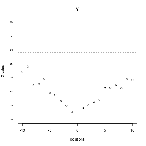
##    aa at         Z       pValue
## 17  M -1 -6.724230 8.826195e-12
## 19  Y -1 -6.707720 9.884452e-12
## 14  Y -2 -6.234550 2.265394e-10
## 29  Y  3 -5.840868 2.596470e-09
## 23  Y  1 -5.816164 3.010664e-09
## 27  Y  2 -5.605347 1.039190e-08
As you can see, we must reject the null hypothesis and declare that the sequence environments of oxidation-prone and oxidation-resistant methionines are distinguishable.
Ploting the differences between sequence environment
The conclusion to which we have just arrived: the oxidable methionines exhibit a differential sequence environment, can be visually illustrated making use of the env.plot() function. For instance, let’s focus on tyrosine, an amino acid that is clearly underrepresented in the environment of MetO.
env.plot(Z[[1]], aa = 'Y', pValue = 0.05)
Other hypothesis that can be easily tested
At this point we’re ready to address a number of different working hypothesis. As an exercise, we suggest the reader to tackle the question of whether the sequence environments of human MetO sites oxidized in vivo and that of MetO sites oxidized in vitro are equal. Would there be differences between prokaryotes and eukaryotes? between plants and animals? and so on.
