Description
Computes changes in the stability of a protein after a residue mutation (ΔΔG), using a force-field approach.
Usage
foldx.mut(pdb, ch , pos, newres = “”, pH = 7, method = "buildmodel", keepfiles = FALSE)
Arguments
pdb the 4-letter identifier of a PDB structure or the path to a PDB file.
ch a letter identifying the chain of interest.
pos the position, in the primary structure, of the residue to be mutated.
newres the one letter code of the residue to be incorporated. When a value is not entered for this parameter, then the function will compute ΔΔG for the mutation to any possible amino acid.
pH a numeric value between 0 and 14.
method a character string specifying the approach to be used; it must be one of ‘buildmodel’, ‘positionscan’.
keepfiles logical, when TRUE the repaired PDB file is saved in the working directory.
Value
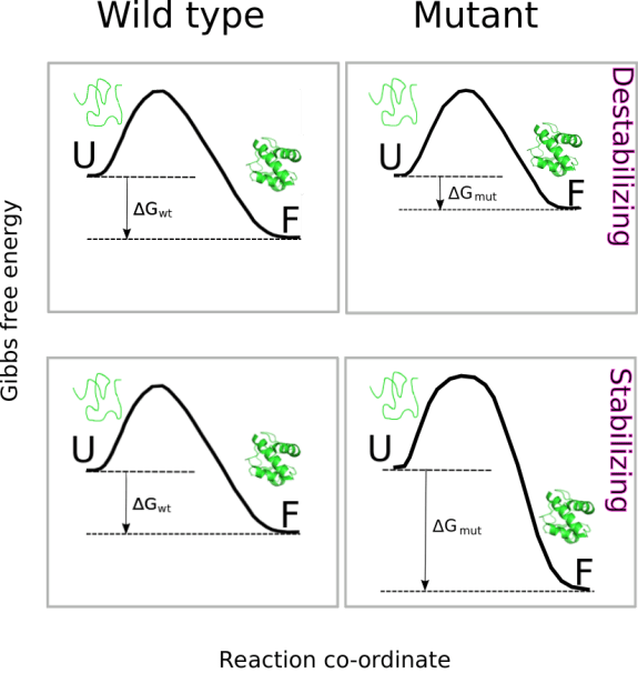
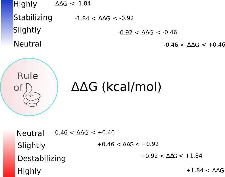
The function computes and returns the ΔΔG (kcal/mol) for the requested residue change, defined as ΔΔG = ΔGmt – ΔGwt, where ΔG is the Gibbs free energy for the folding of the protein from its unfolded state. Thus, a positive value means a destabilizing effect, and vice versa.
References
Schymkowitz et al (2005) Nucl. Ac. Res. 33:W382-W388.
Details
Thermodynamic stability is a fundamental property of proteins that influences protein structure, function, expression, and solubility. Not surprisingly, prediction of the effect of point mutations on protein stability is a topic of great interest in many areas of biological research, including the field of protein post-translational modifications. Consequently, a wide range of strategies for estimating protein energetics has been developed. In the package ptm we have implemented two popular computational approaches for prediction of the effect of amino acid changes on protein stability.
On the one hand, foldx.mut() implements FoldX (buildmodel and positionscan methods), a computational approach that uses a force field method and athough it has been proved to be satisfactorily accurate, it is also a time-consuming method. On the other hand, I-Mutant is a method based on machine-learning and it represents an alternative much faster to FoldX. The ptm function that implements this last approach is imutant().
Although using very different strategies, both functions assess
the thermodynamic stability effect of substituting a single amino acid residue in the protein of interest. To do that, both function perform an estimation of the change in Gibbs free energy, 

Where 


When interpreting results arising from the use of foldx.mut() a practical rule of thumb may be as follows:
To illustrate the use of the functions imutant() and foldx.mut(), we will use as a model the β1 domain of streptococcal protein G (Gβ1), which has been extensively characterized experimentally in terms of thermodynamic stability.
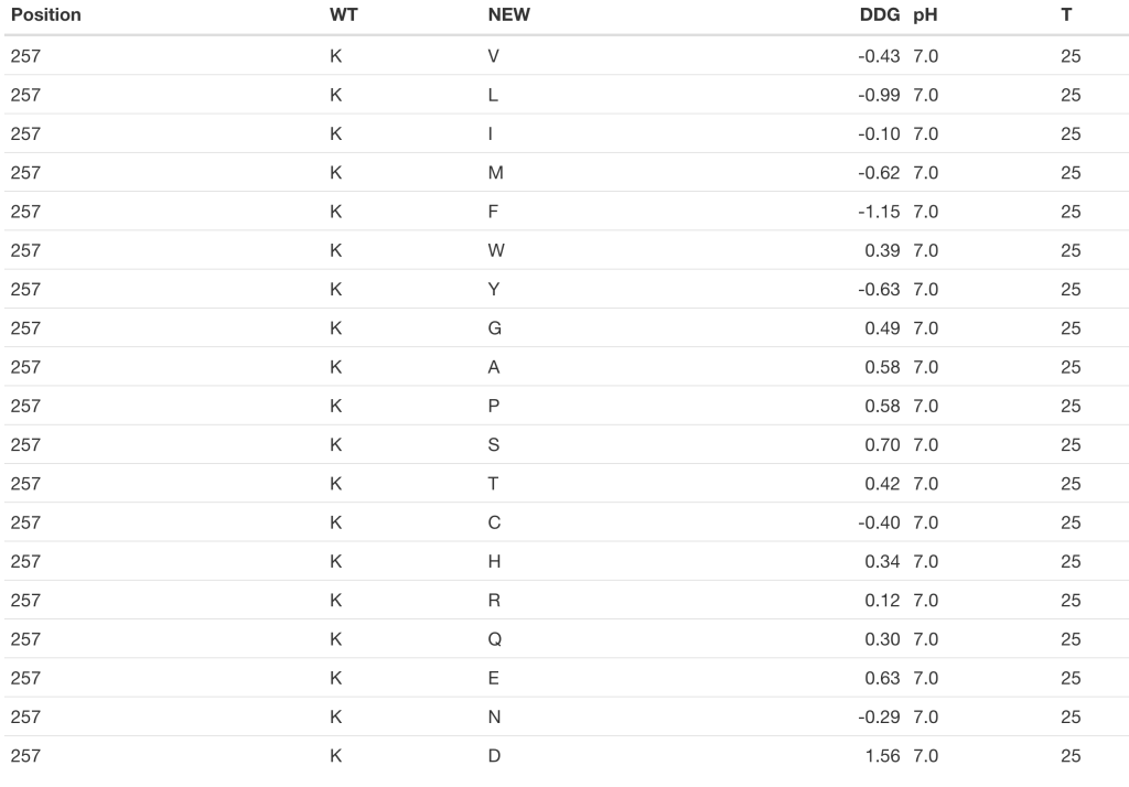
So, let’s start using imutant() to compute the mutational sensitivity, 
GB1_a <- imutant(protein = '1pga', ch = 'A', pos = 31)
kable(GB1_a)

In addition, imutant() allows us to compute the change in stability even if we don’t have 3D structural data, that is, when there is no PDB file for the protein of interest. In this case, we’ll have to pass the primary sequence of the protein as an argument instead of the PDB ID. In the example that concerns us, we must bear in mind that the β1 domain of streptococcal protein G starts at the position 227 of the whole protein sequence:
GB1_b <- imutant(protein = get.seq(pdb2uniprot('1pga', 'A')), pos = 31 + 226)
kable(GB1_b)
We can now compare the results obtained using both approaches: tertiary structure data versus primary structure data:
model <- lm(GB1_b$DDG ~ GB1_a$DDG)
plot(GB1_a$DDG, GB1_b$DDG,
    xlab = expression(paste(Delta, Delta,"G from tertiary structure data", sep = "")),
    ylab = expression(paste(Delta, Delta,"G from primary structure data", sep = "")))
abline(model)

As we can observe, there is a reasonably good correlation between both results (R-squared = 0.7).
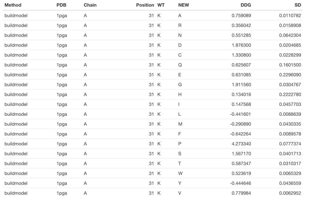
Nevertheless, if the computing time is not a concern for you, then you may wish to use foldx.mut() instead of imutant(). The function foldx.mut() will repair your structure before carrying out the computation. To do that, FoldX identify those residues which have bad torsion angles, or VanderWaals’ clashes, or total energy, and repairs them. The function foldx.mut() will take care of this repair process, so you only have to indicate which of the two alternative methods that foldx.mut() offers you want to use in order to assess the requested change in stability: ‘buildmodel’
GB1_c <- foldx.mut(pdb = '1pga', ch = 'A', pos = 31, method = 'buildmodel')
kable(GB1_c)
or ‘positionscan’.
GB1_d <- foldx.mut(pdb = '1pga', ch = 'A', pos = 31, method = 'positionscan')
kable(GB1_d)
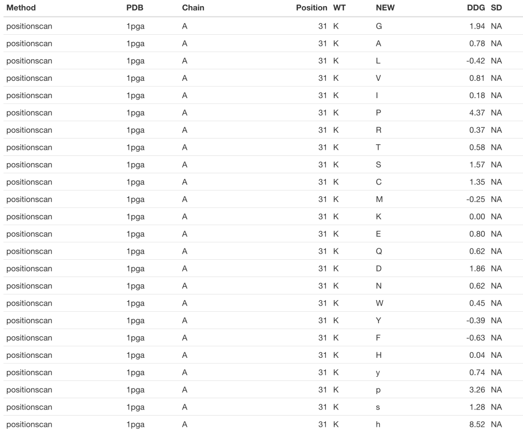
For the details regarding the differences between both methods you would like to consult FoldX’s manual. Nevertheless, at this point you may have already noted that the ‘buildmodel’ method returns a dataframe with 19 raws (one per proteinogenic amino acid alternative to the wild type), while the ‘positionscan’ method returns a dataframe with 24 raws. That is because in addition to the 19 alternative proteinogenic amino acids, this method assess the effect of changing the wild type residue to phosphotyrosine (y), phosphothreonine (p), phosphoserine (s) and hydroxiproline (h).
Now, we can compare the results returned for these two FoldX’s methods:
aa <- ptm:::aai$aa # 20 proteinogenic amino acids
GB1_c <- GB1_c [order(GB1_c $NEW), ]
GB1_d  <- GB1_d[order(GB1_d$NEW), ]
GB1_d <- GB1_d[which(GB1_d$NEW %in% aa), ] # removes PTM residues
GB1_d <- GB1_d[which(GB1_d$NEW != 'K'), ] # This method includes K -> K, DDG = 0

model <- lm(GB1_d$DDG ~ GB1_c$DDG)
plot(GB1_c$DDG, GB1_d$DDG,
      xlab = expression(paste(Delta, Delta,"G (buildmodel)", sep = "")),
      ylab = expression(paste(Delta, Delta,"G (positionscan)", sep = "")))
abline(model)
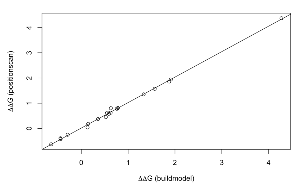
As it can be observed, there is an excellent correlation!
Warning: the function foldx.mut() makes an extensive use of commands invoking the OS, reason why it may not work properly on Windows. If that is your case, you always can use imutant().
