net.go()

Description

Explores the relationship among proteins from a given set

Usage

net.go(data, threshold = 0.2, silent = FALSE)

Arguments

data either a vector containing the UniProt IDs (vertices) or the path to the txt or rda file containing them.

threshold threshold value of the Jaccard index above which two proteins are considered to be linked.

silent logical, if FALSE print details of the running process.

Value

This function first searches the GO for each vertex and then computes the Jaccard index for each protein pair based on their GO terms. Afterwards, an adjacency matrix is computed, where two proteins are linked if their Jaccard index is greater than the selected threshold. The function returns a list containing (i) the dataframe corresponding to the computed Jaccard matrix, (ii) the adjacency matrix, (iii) a vector containing the vertices, and (iv) a matrix describing the edges of the network.

References

Aledo & Aledo (2020) Antioxidants 9(10), 987.

Rhee et al. (2008) Nature Reviews Genetics 9:509–515.

Details

The Gene Ontolory project (GO) provides a controlled vocabulary to describe gene and gene product attributes. Thus, a GO annotation is a statement describing some biological aspect. GO annotations are created by associating a gene or gene product with a GO term. Together, these statements comprise a “snapshot” of current biological knowledge. Hence, GO annotations capture statements about three disjoint categories: cellular component, molecular function and biological process. In this way, GO terms, using a controlled and hierarchical vocabulary, help to describe how a gene functions at the molecular level, where in the cell it functions, and what biological processes it helps to carry out.

The use of this vocabulary (GO annotations) has diverse applications, perhaps the most popular of them is the functional profiling. The goal of functional profiling is to determine which processes might be different in particular sets of genes (or gene products). That is, GO annotations are used to determine which biological processes, functions, and/or locations are significantly over- or under-represented in a given group of genes (or gene products). This approach is also known as GO term enrichment analysis.

Another popular application of GO annotations is GO network analysis, that we address herein. To formalize the analysis, we began by defining the sets P and O in the following way.

$P := \{$ UniProt ID of the proteins of interest $\}$

$O := \{$ GO terms of the proteins from the species of interest $\}$

That is, P is going to be the set of all the proteins we want to analyze. Each element from P is identified by its corresponding UniProt ID. For instance, let’s P be the set of all human proteins containing methionine sulfoxide (MetO) after an oxidative challenge to the cell. On the other hand, O is formed by all the GO terms of human proteins. In this way, we can define the function f as follows:

$f : P \to \wp(O)$

$p \mapsto f(p) = \{$ GO terms annotated to protein p $\}$

where $\wp(O)$ is the powerset of O; that is, the set formed by all the subsets of O. In this way, we are ready to define an endorelation over the set P. For this purpose, we will say that $p_i$ and $p_j$ are related, which is denoted as $p_i \Re p_j$ , if and only if $p_i$ and $p_j$ share at least a certain percent of its GO terms. In other words, if their Jaccard similarity index is equal or greater than a given threshold.

$\begin{aligned} \frac{\vert f(p_i) \bigcap f(p_j) \vert}{\vert f(p_i) \bigcup f(p_j) \vert} \geq threshold \end{aligned}$

Formally, a graph $G(V, E)$ is a mathematical structure consisting of a set of vertices, V, and a set of edges, E, where its elements are unordered pairs, $(a, b) \in V$ . In our case, we are going to build and analyze the following graph:

$G = (V = P, E = \{(p_i, p_j) \in P x P : p_i \Re p_j \}$

Thus, our first goal is to get the set we have called P:

sites <- meto.search(organism = 'Homo sapiens',
                     oxidant = 'hydrogen peroxide')
P <- unique(sites$prot_id[which(sites$met_vivo_vitro == "vivo")])

Once we have the set P, we are ready to use the function net.go():

network <- net.go(P, threshold = 0.5, silent = TRUE)

This function first searchs the GO terms for each node (protein in P) and then computes the Jaccard index for each protein pair based on their GO terms. Afterwards, an adjacency matrix is computed, where two proteins are linked if their Jaccard index is greater than the selected threshold.

Let’s examine the first 10 columns and rows from the Jaccard matrix we have obtained:

Jaccard <- network[[1]]
Jaccard[1:10, 1:10]

##        A2RRP1 A3KN83 A5YKK6 A6NEC2 A6NIZ1 A8K0Z3 A8MWD9 B0I1T2 O00116 O00161
## A2RRP1     NA      0  0.071  0.045  0.150  0.100  0.000  0.043  0.071  0.075
## A3KN83     NA     NA  0.025  0.000  0.000  0.000  0.040  0.000  0.000  0.000
## A5YKK6     NA     NA     NA  0.022  0.070  0.063  0.039  0.029  0.082  0.048
## A6NEC2     NA     NA     NA     NA  0.043  0.023  0.000  0.043  0.000  0.048
## A6NIZ1     NA     NA     NA     NA     NA  0.071  0.000  0.089  0.069  0.073
## A8K0Z3     NA     NA     NA     NA     NA     NA  0.000  0.061  0.061  0.083
## A8MWD9     NA     NA     NA     NA     NA     NA     NA  0.000  0.000  0.000
## B0I1T2     NA     NA     NA     NA     NA     NA     NA     NA  0.018  0.078
## O00116     NA     NA     NA     NA     NA     NA     NA     NA     NA  0.062
## O00161     NA     NA     NA     NA     NA     NA     NA     NA     NA     NA

As expected, we note that Jaccard is an upper triangular matrix. Now we also examine the first rows and columns from the adjacency matrix:

Adjacency <- network[[2]]
Adjacency[1:10, 1:10]

##        A2RRP1 A3KN83 A5YKK6 A6NEC2 A6NIZ1 A8K0Z3 A8MWD9 B0I1T2 O00116 O00161
## A2RRP1      0      0      0      0      0      0      0      0      0      0
## A3KN83      0      0      0      0      0      0      0      0      0      0
## A5YKK6      0      0      0      0      0      0      0      0      0      0
## A6NEC2      0      0      0      0      0      0      0      0      0      0
## A6NIZ1      0      0      0      0      0      0      0      0      0      0
## A8K0Z3      0      0      0      0      0      0      0      0      0      0
## A8MWD9      0      0      0      0      0      0      0      0      0      0
## B0I1T2      0      0      0      0      0      0      0      0      0      0
## O00116      0      0      0      0      0      0      0      0      0      0
## O00161      0      0      0      0      0      0      0      0      0      0

Not surprisingly, this submatrix is the zero matrix. That is, any of the 10 first proteins are related among them according to our criteria (threshold = 0.5). Nevertheless, we can check that our graph will have 578 edges (pairs of related proteins):

edges <- network[[4]]
nrow(edges)

## [1] 578

head(edges)

##      [,1]     [,2]    
## [1,] "A3KN83" "O15037"
## [2,] "A5YKK6" "Q9NZN8"
## [3,] "A6NEC2" "O75976"
## [4,] "A6NEC2" "Q5JRX3"
## [5,] "A6NEC2" "Q9NZ08"
## [6,] "A6NIZ1" "P84085"

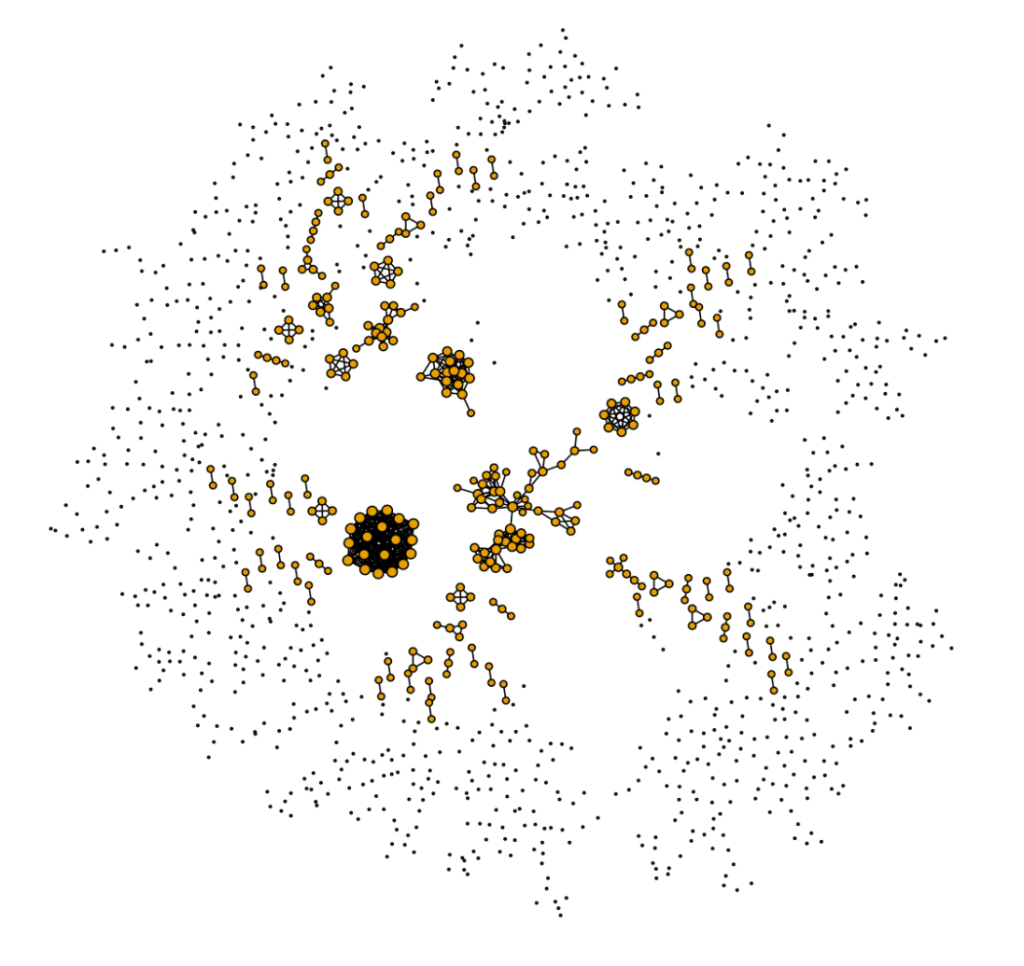
Now, if we have previously installed the package igraph, then we are in conditions to plot our network:

G <- igraph::graph_from_data_frame(d = edges, 
                                   vertices = network[[3]],
                                   directed = FALSE)
plot(G, 
     vertex.label = NA,
     edge.color = "black",
     vertex.size = 0.5 + (igraph::degree(G))^(1/5),
     layout = igraph::layout_components(G)
    )