Description
Represents the values of a property and show the PTM sites along a protein sequence
Usage
ptm.plot(up_id, pdb = “”, property, ptm, dssp = 'compute', window = 1, sdata = TRUE, …)
Arguments
up_id a character string for the UniProt ID of the protein of interest.
pdb Optional argument to indicate the PDB and chain to be used (i.e. ‘1u8f.O’). If we leave this argument empty, the function will make the election for us whenever possible.
property a character string indicating the property of interest. It should be one of ‘sasa’, ‘acc’, ‘dpx’, ‘entropy7.aa’,’entropy7.codon’, ‘entropy100.aa’, ‘entropy100.codon’, ‘eiip’, ‘volume’, ‘polarizability’, ‘av.hyd’, ‘pi.hel’, ‘a.hel’, ‘b.sheet’, ‘B.factor’, or ‘own’.
ptm a character vector indicating the PTMs of interest. It should be among: ‘ac’ (acetylation), ‘me’ (methylation), ‘meto’ (sulfoxidation), ‘p’ (phosphorylation), ‘ni’ (nitration), ‘su’ (sumoylation) or ‘ub’ (ubiquitination), ‘gl’ (glycosylation), ‘sni’ (S-nitrosylation),’reg’ (regulatory), ‘dis’ (disease).
dssp character string indicating the method to compute DSSP. It should be either ‘compute’ or ‘mkdssp’.
window positive integer indicating the window size for smoothing with a sliding window average (default: 1, i.e. no smoothing).
sdata logical, if TRUE save a Rda file with the relevant data in the current directory.
Value
This function returns either one or two plots related to the chosen property along the primary structure, as well as the computed data if sdata has been set to TRUE.
See Also
find.aaindex()
Details
This function returns a plot related to the choosen property along the primary structure.
Currently the supported properties are:
- sasa: Solvent-accessible surface area (3D)
- acc: Accessibility (3D)
- dpx: Depth (3D)
- volume: Normalized van der Waals volume (1D)
- mutability: Relative mutability, Jones 1992, (1D)
- helix: Average relative probability of helix, Kanehisa-Tsong 1980,(1D)
- beta-sheet: Average relative probability of beta-sheet, Kanehisa-Tsong 1980, (1D)
- pi-helix: Propensity of amino acids within pi-helices, Fodje-Al-Karadaghi 2002, (1D)
- hydropathy: Hydropathy index, Kyte-Doolittle 1982, (1D)
- avg.hyd: Normalized average hydrophobicity scales, Cid et al 1992, (1D)
- hplc: Retention coefficient in HPLC at pH7.4, Meek 1980, (1D)
- argos: Hydrophobicity index, Argos et al 1982, (1D)
- eiip: Electron-ion interaction potential, Veljkovic et al 1985, (1D)
- polarizability: Polarizability parameter, Charton-Charton 1982, (1D)
- entropy7.aa: Shannon entropy based on 7 species and protein sequences (EVO)
- entropy100.aa: Shannon entropy based on 100 species and protein sequences (EVO)
- entropy7.condon: Shannon entropy based on 7 species and codon sequences (EVO)
- entropy100.codon: Shannon entropy based on 100 species and codon sequences (EVO)
For 3D properties such as sasa, acc or dpx, for which different values can be obtained depending on the cuaternary structure, we first compute the property value for each residue in the whole protein and plotted it against the residue position. Then, the values for this property are computed in the isolated chain (a single polypeptide chain) and in a second plot, the differences between the values in the whole protein and the chain are plotted against the residue position.
The selected PTM sites are also pointed in the same plot. Currently the supported PTM are:
- Acetylation (ac)
- Disease (dis)
- Glycosylation (gl)
- Methylation (me)
- Nitration (ni)
- Phosphorylation (p)
- Regulatory (reg)
- S-nitrosylation (sni)
- Sulfoxidation (meto)
- Sumoylation (su)
- Ubiquitination (ub)
Let’s look at an example using glyceraldehyde-3-phosphate dehydrogenase (P04406), a homotetrameric protein. We choose methionine sulfoxidation as PTM and a hydrophobicity index as the property to be plotted along the primary sequence.
ptm.plot(up_id = "P04406", property = 'avg.hyd', ptm = 'meto')
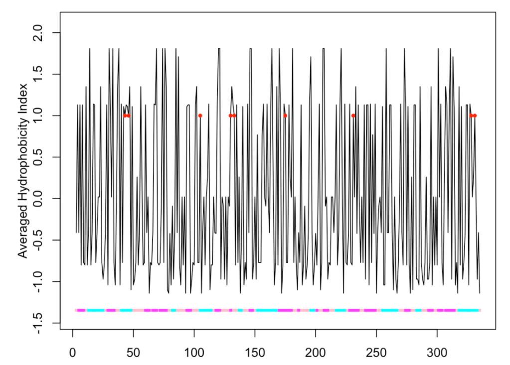
## [1] "Work done."
## attr(,"uniprot")
## [1] "P04406"
## attr(,"pdb")
## [1] "1u8f"
## attr(,"chain")
## [1] "O"
Herein, we are using window = 1 (the default value), at each position we plot the index value of the residue found at that position. Therefore, since the modified residues (red circles) are always methionines, the ordinates values at the corresponding positions are always the same (the value for methionine). Furthermore, the plot exhibits very sharp picks. More often we will be interested in knowing if the modified residues are placed in hydrophobic regions. In these cases, we can use a sliding window to compute the ordinate values.
ptm.plot(up_id = "P04406", property = 'avg.hyd', ptm = 'meto', window = 5)

## [1] "Work done."
## attr(,"uniprot")
## [1] "P04406"
## attr(,"pdb")
## [1] "1u8f"
## attr(,"chain")
## [1] "O"
Now we have obtain a smoother plot and more interestingly, we observe that the oxidized methionines are distributed through regions of different hydrophobicity. We can also observe that the plot shows, at the bottom, a bar indicating the secondary structure coded with different colors (cyan for helices, magenta for sheets and pink for loops).
Of course, we can combine different PTMs:
ptm.plot(up_id = "P04406", property = 'avg.hyd',
         ptm = c('meto', 'p', 'ac'), window = 5)
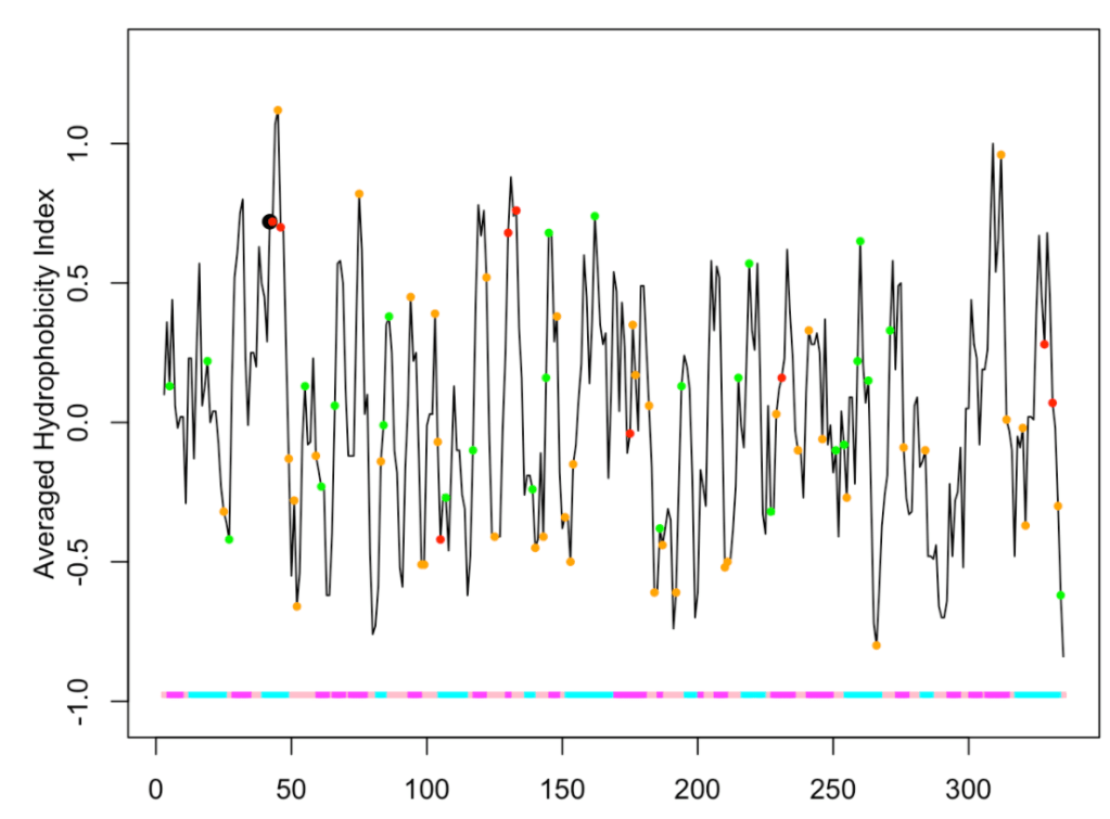
## [1] "Work done."
## attr(,"uniprot")
## [1] "P04406"
## attr(,"pdb")
## [1] "1u8f"
## attr(,"chain")
## [1] "O"
The phosphorylation, acetylation and sulfoxidation positions are shown as orange, green and red circles, respectively. We observe at position 42 a black circle of higher diameter, which indicates that the residue (tyrosine) found at that position can suffer different PTMs. In this case phosphorylation and acetylation. If you didn’t turn the argument sdata to FALSE, you can explore the data.
load("./plotptm_cache/scan_P04406.Rda")
knitr::kable(scan[1:10, ])
| id | n | aa | meto | p | ac | me | ub | su | gl | sni | ni | reg | dis | multi | |
|---|---|---|---|---|---|---|---|---|---|---|---|---|---|---|---|
| 5 | P04406 | 5 | K | NA | NA | TRUE | TRUE | TRUE | NA | NA | NA | NA | NA | NA | 3 |
| 13 | P04406 | 13 | R | NA | NA | NA | TRUE | NA | NA | NA | NA | NA | NA | NA | 1 |
| 19 | P04406 | 19 | T | NA | NA | TRUE | NA | TRUE | NA | NA | NA | NA | NA | NA | 2 |
| 25 | P04406 | 25 | S | NA | TRUE | NA | NA | NA | NA | NA | NA | NA | NA | NA | 1 |
| 27 | P04406 | 27 | K | NA | NA | TRUE | NA | TRUE | NA | NA | NA | NA | NA | NA | 2 |
| 42 | P04406 | 42 | Y | NA | TRUE | TRUE | NA | TRUE | NA | NA | NA | NA | TRUE | NA | 3 |
| 43 | P04406 | 43 | M | TRUE | NA | NA | NA | NA | NA | NA | NA | NA | NA | NA | 1 |
| 45 | P04406 | 45 | Y | NA | TRUE | NA | NA | NA | NA | NA | NA | NA | NA | NA | 1 |
| 46 | P04406 | 46 | M | TRUE | NA | NA | NA | NA | NA | NA | NA | NA | TRUE | NA | 1 |
| 49 | P04406 | 49 | Y | NA | TRUE | NA | NA | NA | NA | NA | NA | NA | NA | NA | 1 |
The color code used for the PTMs is:
- Acetylation (ac): green.
- Disease (dis): darkseagreen3.
- Glycosylation (gl): purple.
- Methylation (me): aquamarine.
- Nitration (ni): blue.
- Phosphorylation (p): orange.
- Regulatory (reg): deepskyblue4.
- S-nitrosylation (sni): yellow.
- Sulfoxidation (meto): red.
- Sumoylation (su): deeppink.
- Ubiquitination (ub): darkgreen.
Similarly, for the secundary structure elements:
load("./plotptm_cache/sse_1u8f.Rda")
knitr::kable(head(sse))
| resnum | respdb | chain | aa | ss | sasa_complex | sasa_chain | delta_sasa | acc_complex | acc_chain | delta_acc |
|---|---|---|---|---|---|---|---|---|---|---|
| 1 | 3 | O | K | C | 186 | 186 | 0 | 0.882 | 0.882 | 0 |
| 2 | 4 | O | V | C | 9 | 9 | 0 | 0.056 | 0.056 | 0 |
| 3 | 5 | O | K | E | 98 | 98 | 0 | 0.464 | 0.464 | 0 |
| 4 | 6 | O | V | E | 0 | 0 | 0 | 0.000 | 0.000 | 0 |
| 5 | 7 | O | G | E | 0 | 0 | 0 | 0.000 | 0.000 | 0 |
| 6 | 8 | O | V | E | 0 | 0 | 0 | 0.000 | 0.000 | 0 |
Let’s now try to plot a 3D property, for instance, the accessibility of the residue to the solvent.
ptm.plot(up_id = "P04406", property = 'acc', ptm = 'meto')
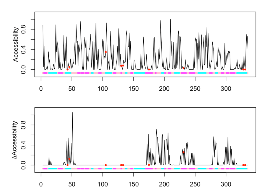
## [1] "Work done."
## attr(,"uniprot")
## [1] "P04406"
## attr(,"pdb")
## [1] "1u8f"
## attr(,"chain")
## [1] "O"
As expected, we obtain two plots. One with the accessibility of each residue when considered in the context of the whole protein (the tetramer), and a second plot showing the increase in accessibility when a single monomer is considered. Thus, the picks in this second plot represent those residues that are forming part of the subunit-subunit interfaces. Three MetO are found within these regions (at positions 43, 46 and 231).
Now, we are going to plot an evolutionary property, for instance the Shannon entropy:
ptm.plot(up_id = "P04406", property = 'entropy100.aa', ptm = 'meto')
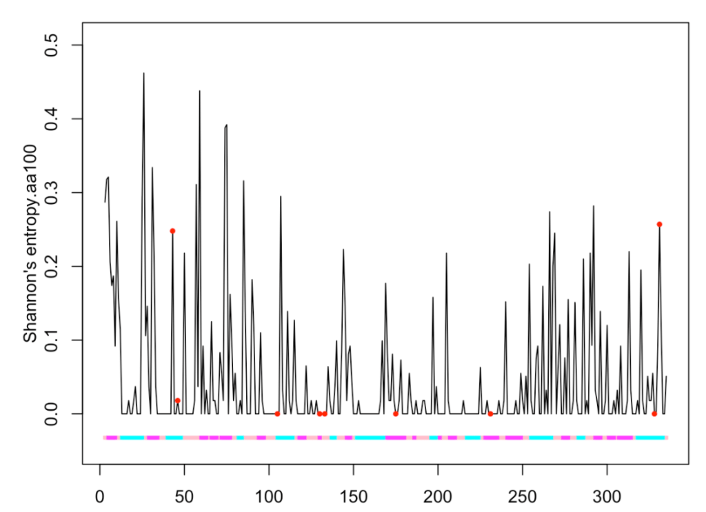
## [1] "Work done."
## attr(,"uniprot")
## [1] "P04406"
## attr(,"pdb")
## [1] "1u8f"
## attr(,"chain")
## [1] "O"
We observe that six methionine residues (at positions 105, 130, 133, 175, 231 and 328) are conserved throughout the sequences of 100 different species.
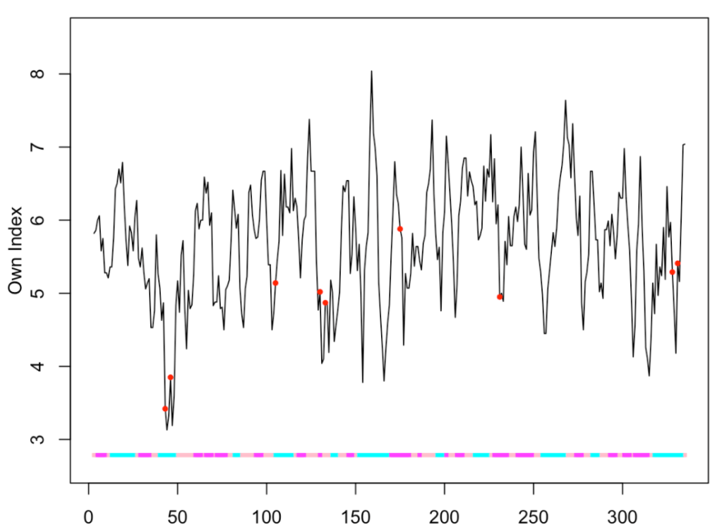
What if we want to use a different property than those listed above? For instance, suppose we wish to plot the frequency in human proteins of the amino acid found at each position.
f <- c(7.00, 5.63, 3.60, 4.75, 2.30, 4.76, 7.09, 6.58, 2.62, 4.36,
       9.96, 5.73, 2.14, 3.67, 6.28, 8.31, 5.36, 1.22, 2.68, 5.99)
names(f) <- c('A', 'R', 'N', 'D', 'C', 'Q', 'E', 'G', 'H', 'I',
              'L', 'K', 'M', 'F', 'P', 'S', 'T', 'W', 'Y', 'V')
ptm.plot(up_id = "P04406", property = 'own', ptm = 'meto', window = 5, index = f)
## [1] "Work done."
## attr(,"uniprot")
## [1] "P04406"
## attr(,"pdb")
## [1] "1u8f"
## attr(,"chain")
## [1] "O"
More than 500 different amino acid indices have been described. If you want to use some of them, ptm provides a useful function that will help you to find the desired index. Let’s say we are interested in the number of hydrogen bond donors, then we could use the keyword ‘hydrogen bond’ as argument for the function find.aaindex():
find.aaindex('hydrogen bond')
## FAUJ880109
##         86
This function returns the ID of the index of interest, but we can easily have more detailed information as follows:
bio3d::aa.index[[find.aaindex('hydrogen bond')]]$D
## [1] "Number of hydrogen bond donors (Fauchere et al., 1988)"
If that is the index we wanted, now we can proceed as follows:
ptm.plot(up_id = "P04406",
         property = 'own',
         ptm = 'meto',
         window = 5,
         index = bio3d::aa.index[[find.aaindex('hydrogen bond')]]$I)

## [1] "Work done."
## attr(,"uniprot")
## [1] "P04406"
## attr(,"pdb")
## [1] "1u8f"
## attr(,"chain")
## [1] "O"
We can also search for an index using the author as keyword:
find.aaindex("Levit")
## LEVM760101 LEVM760102 LEVM760103 LEVM760104 LEVM760105 LEVM760106
##        153        154        155        156        157        158
## LEVM760107 LEVM780101 LEVM780102 LEVM780103 LEVM780104 LEVM780105
##        159        160        161        162        163        164
## LEVM780106 KOEP990101 KOEP990102
##        165        454        455
To obtain further details:
lapply(find.aaindex("Levit"), function(x) bio3d::aa.index[[x]]$D)
## $LEVM760101
## [1] "Hydrophobic parameter (Levitt, 1976)"
##
## $LEVM760102
## [1] "Distance between C-alpha and centroid of side chain (Levitt, 1976)"
##
## $LEVM760103
## [1] "Side chain angle theta(AAR) (Levitt, 1976)"
##
## $LEVM760104
## [1] "Side chain torsion angle phi(AAAR) (Levitt, 1976)"
##
## $LEVM760105
## [1] "Radius of gyration of side chain (Levitt, 1976)"
##
## $LEVM760106
## [1] "van der Waals parameter R0 (Levitt, 1976)"
##
## $LEVM760107
## [1] "van der Waals parameter epsilon (Levitt, 1976)"
##
## $LEVM780101
## [1] "Normalized frequency of alpha-helix, with weights (Levitt, 1978)"
##
## $LEVM780102
## [1] "Normalized frequency of beta-sheet, with weights (Levitt, 1978)"
##
## $LEVM780103
## [1] "Normalized frequency of reverse turn, with weights (Levitt, 1978)"
##
## $LEVM780104
## [1] "Normalized frequency of alpha-helix, unweighted (Levitt, 1978)"
##
## $LEVM780105
## [1] "Normalized frequency of beta-sheet, unweighted (Levitt, 1978)"
##
## $LEVM780106
## [1] "Normalized frequency of reverse turn, unweighted (Levitt, 1978)"
##
## $KOEP990101
## [1] "Alpha-helix propensity derived from designed sequences (Koehl-Levitt, 1999)"
##
## $KOEP990102
## [1] "Beta-sheet propensity derived from designed sequences (Koehl-Levitt, 1999)"
If we choose to plot the side chain torsion angle phi:
ptm.plot(up_id = "P04406",
         property = 'own',
         ptm = 'meto',
         window = 5,
         index = bio3d::aa.index[[find.aaindex('Levit')[4]]]$I)

## [1] "Work done."
## attr(,"uniprot")
## [1] "P04406"
## attr(,"pdb")
## [1] "1u8f"
## attr(,"chain")
## [1] "O"
