In the large inventory of the benefits provided by the presence of a sulfur atom in the side chain of methionine, we can find those effects derived from the so-called S-aromatic motifs. Indeed, an interaction of methionine and nearby aromatic residues (Phe, Tyr and Trp) was described as early as in the mid-eighties. Even earlier, a frequency of sulfur and aromatic ring in close proximity within proteins higher than expected had been noticed. Despite the potential importance of these findings, they went largely overlooked, perhaps because the physicochemical nature of this bond is only poorly understood.
Although the strength of these interactions may depend on the conditions of its environment, it is accepted that the S-aromatic interaction occurs at a greater distance (5-7 Å) than a salt bridge (< 4 Å), while the energies associated with either interaction are comparable. More recently, extensive surveys of the Protein Data Bank have revealed the importance of the methionine-aromatic motif for stabilizing protein structures and for protein-protein interactions (see the review Methionine in proteins: The Cinderella of the proteinogenic amino acids for further details).
When searching for S-aromatic motifs in proteins, two relevant variables are the distance between the delta sulfur atom (SD) and the centroid of the aromatic ring, which can be computed as the euclidean norm of the vector 

The other relevant variable is the angle theta. This angle is defined as that between the sulfur-aromatic vector (


Note that two extreme cases are possible: a face-on interaction (angles around 0º) and an edge-on interaction (involving angles around 90º).
Currently, the ptm package offers three functions that may be useful for the study of these S-aromatic motifs:
To illustrate the use of these functions we are going to use calmodulin (CaM) as a model protein. Calmodulin is a multifunctional calcium-binding protein expressed in all eukaryotic cells. The binding of the secondary messenger Ca2+ to CaM changes the CaM conformation and its affinity for its various targets. Methionine residues of CaM play an essential role in the sequence-independent specific binding to its many protein targets. In a Ca2+ free medium, CaM exhibits a spatial conformation corresponding to the so-called apoCaM (PDB ID: 1CFD). On the other hand, when CaM binds two Ca2+ ions, the protein adopts a different spatial conformation corresponding to the holoCaM (PDB ID: 1CLL).
If we pass the PDB ID of the apoCaM to the function saro.motif(pdb = ‘1cfd’, threshold = 6), and we place the output in an object we may call apo_cam, we can observe that this form of the calmodulin exhibits 8 S-aromatic motifs close to the edge-on type.
library(knitr)
kable(apo_cam)
| Met | Aromatic | Length | Angle | |
|---|---|---|---|---|
| 2 | MET-A-36 | PHE-A-68 | 5.73 | 86.73 |
| 5 | MET-A-72 | PHE-A-12 | 4.83 | 83.08 |
| 6 | MET-A-72 | PHE-A-68 | 4.34 | 84.13 |
| 7 | MET-A-76 | PHE-A-12 | 5.77 | 89.13 |
| 8 | MET-A-109 | PHE-A-89 | 5.98 | 90.48 |
| 9 | MET-A-109 | PHE-A-141 | 4.93 | 84.61 |
| 10 | MET-A-124 | PHE-A-141 | 5.82 | 91.09 |
| 11 | MET-A-144 | PHE-A-141 | 4.67 | 96.94 |
If we repeat the process, but now for the holoCaM (PDB ID 1CLL):
kable(holo_cam)
| Met | Aromatic | Length | Angle | |
|---|---|---|---|---|
| 2 | MET-A-36 | PHE-A-19 | 6.98 | 90.1 |
| 4 | MET-A-71 | PHE-A-68 | 5.82 | 95 |
| 5 | MET-A-72 | PHE-A-12 | 6.1 | 88.85 |
| 6 | MET-A-72 | PHE-A-68 | 4.72 | 96.31 |
| 7 | MET-A-76 | PHE-A-12 | 6.57 | 91.55 |
| 8 | MET-A-109 | PHE-A-92 | 6.43 | 89.01 |
| 11 | MET-A-145 | PHE-A-141 | 4.65 | 83.2 |
These tables show a dynamic remodeling of the S-aromatic bonds dependent on calcium ions, which is better summarized in the form of a network graph:

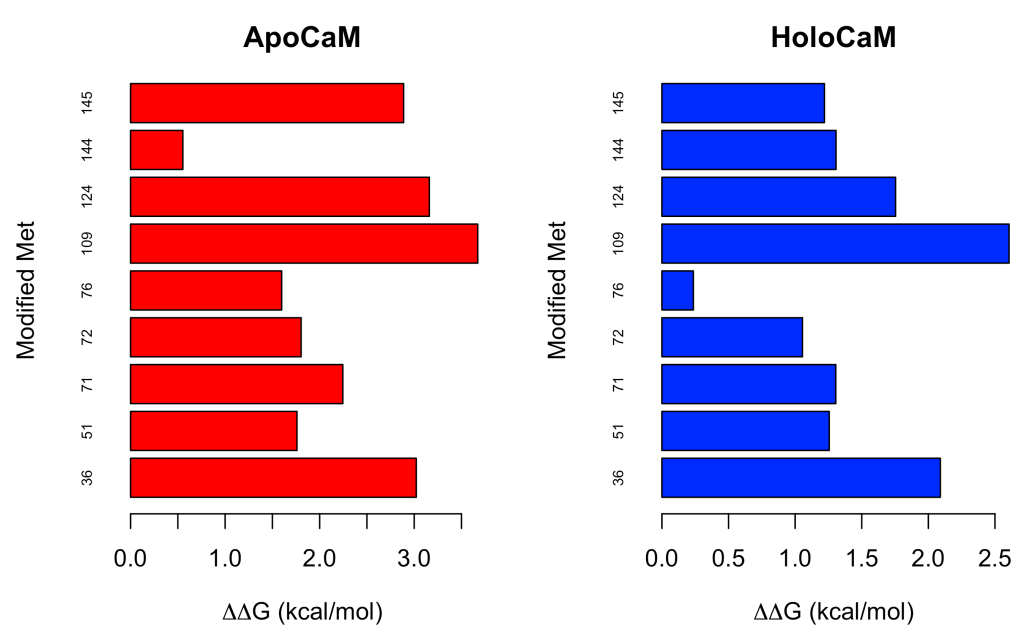
The information provided by this dynamic network can be complemented using the function ddG.ptm(), which will inform us about the changes in thermodynamic stability caused by modification of the corresponding methionine residues.
To this end, we need the UniProt ID of human calmodulin-1, which is P0DP23. Nevertheless, if all we know is that we are interested in human calmodulin-1, and we don’t want to leave the R IDE to search the desired identifier, we can make use of the function meto.list(), typing:
id <- meto.list('Calmodulin-1')$prot_id[which(meto.list('Calmodulin-1')$prot_sp == 'Homo sapiens')]
Now we get the amino acid sequence of this protein:
seq <- get.seq(id) # CaM sequence
seq <- substring(seq, 2, nchar(seq)) # Removing the initiation methionine
met <- gregexpr("M", seq)[[1]] # Positions at which methionines are found
Once we know at which positions the protein exhibits a methionine residue, we are in conditions to compute the change in free energy after modifying those residues. To this end, the arguments taken by the ddG.ptm() functions are the PDB ID of interest, the position of the residue to be modified, and the type of post-translation modification to be introduced. In our case, we set ptm = ‘MetO-Q’ that, as explained somewhere else, mimics the sulfoxidation of methionine.
meto_apo <- lapply(met, function(x) ddG.ptm('1cfd', pos = x, 'A', ptm = 'MetO-Q'))
meto_apo <- round(as.numeric(unlist(meto_apo)), 3)

meto_holo <- lapply(met, function(x) ddG.ptm('1cll', pos = x, 'A', ptm = 'MetO-Q'))
meto_holo <- round(as.numeric(unlist(meto_holo)), 3)
The objects meto_apo and meto_halo contain the Gibbs free energy change values in kcal/mol. Now, let’s plot them:
oldpar <- par()
par(mfrow=c(1,2))
on.exit(oldpar)
barplot(meto_apo,
        horiz = TRUE, names.arg = met, cex.names = 0.6,
        xlab = expression(paste(Delta, Delta, "G (kcal/mol)", sep = "")),
        ylab = "Modified Met",
        col = "red",
        main = "ApoCaM")

barplot(meto_holo,
        horiz = TRUE, names.arg = met, cex.names = 0.6,
        xlab = expression(paste(Delta, Delta, "G (kcal/mol)", sep = "")),
        ylab = "Modified Met",
        col = "blue",
        main = "HoloCaM")
If we want to obtain a greater wealth of raw data related to the inter-residual distances between the sulfur atom and the aromatic ring, we can choose the function saro.dist()
raw_data <- saro.dist('1cfd', rawdata = TRUE)
## Note: Accessing on-line PDB file
The output of this function is a list of two elements. The first is a dataframe where each row is a methionine residue. For each methionine residue this dataframe provides the identity of the closest tyrosine, phenylalanine and tryptophan, as well as the corresponding distances in ångströms. Also, the number of S-aromatic bonds that each methionine residue forms with tyrosine, phenylalanine and tryptophan is provided.
closest <- raw_data[[1]]
kable(closest[,1:7])
| Met | Tyr_closest | Yd | number_bonds_MY | Phe_closest | Fd | number_bonds_MF |
|---|---|---|---|---|---|---|
| MET-A-36 | TYR-A-138 | 31.34600 | 0 | PHE-A-68 | 5.729923 | 1 |
| MET-A-51 | TYR-A-138 | 32.35663 | 0 | PHE-A-68 | 9.254798 | 0 |
| MET-A-71 | TYR-A-138 | 33.66811 | 0 | PHE-A-68 | 6.748291 | 1 |
| MET-A-72 | TYR-A-138 | 29.66193 | 0 | PHE-A-68 | 4.337354 | 2 |
| MET-A-76 | TYR-A-138 | 23.06316 | 0 | PHE-A-12 | 5.767916 | 1 |
| MET-A-109 | TYR-A-138 | 10.51135 | 0 | PHE-A-141 | 4.932660 | 2 |
| MET-A-124 | TYR-A-138 | 14.29151 | 0 | PHE-A-141 | 5.822773 | 1 |
| MET-A-144 | TYR-A-138 | 12.72373 | 0 | PHE-A-141 | 4.668086 | 1 |
| MET-A-145 | TYR-A-138 | 11.57210 | 0 | PHE-A-89 | 6.869048 | 1 |
The second one is a dataframe where each row corresponds to a methionine residue and each column provides the distance in ångströms to the indicated aromatic residue. There will be as many columns as aromatic residues are found in the given protein.
all_distances <- raw_data[[2]]
kable(all_distances[, 1:9])
| Met | TYR-A-99 | TYR-A-138 | PHE-A-12 | PHE-A-16 | PHE-A-19 | PHE-A-65 | PHE-A-68 | PHE-A-89 | |
|---|---|---|---|---|---|---|---|---|---|
| MET-A-36 | MET-A-36 | 38.34729 | 31.34600 | 8.226976 | 10.728714 | 11.24757 | 11.843919 | 5.729923 | 29.521469 |
| MET-A-51 | MET-A-51 | 38.77071 | 32.35663 | 12.838687 | 13.658764 | 15.85700 | 14.983522 | 9.254798 | 31.477093 |
| MET-A-71 | MET-A-71 | 40.04736 | 33.66811 | 11.430481 | 10.568579 | 14.30609 | 11.952324 | 6.748291 | 32.451932 |
| MET-A-72 | MET-A-72 | 36.51362 | 29.66193 | 4.832751 | 9.607086 | 12.52884 | 8.912004 | 4.337354 | 27.613016 |
| MET-A-76 | MET-A-76 | 30.04367 | 23.06316 | 5.767916 | 15.547118 | 18.02415 | 12.868828 | 10.857783 | 20.779809 |
| MET-A-109 | MET-A-109 | 14.97264 | 10.51135 | 26.156675 | 36.374170 | 38.54434 | 32.058028 | 32.674068 | 5.977779 |
| MET-A-124 | MET-A-124 | 18.12148 | 14.29151 | 24.387935 | 34.057192 | 37.27113 | 29.249233 | 30.911524 | 10.376882 |
| MET-A-144 | MET-A-144 | 14.83339 | 12.72373 | 26.724114 | 36.179474 | 40.12319 | 31.327583 | 32.806115 | 10.739657 |
| MET-A-145 | MET-A-145 | 17.20407 | 11.57210 | 21.969612 | 32.146813 | 34.53947 | 27.809736 | 28.500331 | 6.869048 |
Finally, if we are interested in a particular pair of residues, let’s say M76 and F12, we can use:
kable(saro.geometry('1cll', rA = 12, rB = 76))
##   Note: Accessing on-line PDB file
##    PDB has ALT records, taking A only, rm.alt=TRUE
| resid | chain | resno | x | y | z | length | theta |
|---|---|---|---|---|---|---|---|
| MET | A | 76 | 6.184 | 27.197 | 19.856 | NA | NA |
| PHE | A | 12 | 0.484 | 29.837 | 21.784 | 6.570904 | 91.55 |
where x, y and z are the Cartesian coordinates of either the sulfur delta of methionine or the centroid of the aromatic ring.
